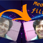
Image processing encompasses a series of techniques that are applied to images in order to “clean” them of possible artifacts that may hinder their subsequent analysis. This is very important because, for example, the decision making of an AI algorithm can vary depending on the quality of the image it receives as input.
In this post I will show you to correct the noise artifact known as ‘Salt & Pepper’. Its name is given because only a few pixels are noisy, but they are very noisy, where ‘salt’ correspond with white pixels and ‘pepper’ with the black ones.

In the image above, we can hardly recognize that it is a woman because of the large amount of noise, and that would also be a problem for any image classifier algorithm. This problem is what we are going to solve by applying the median filter.
Median filter
We will use a median filter that will run through the image to correct the anomalous pixel values. This filter is ideal for eliminating unipolar or bipolar impulsive random noise, as is, in the latter case, the case of the noise called “salt and pepper”. On the other hand, image contrast is lost due to the filter’s own work, and in case of not choosing a good value for the kernel window size, this effect will be exacerbated, or else it will not remove the noise at all.
How does it work?
The median filter replaces each pixel with the median of the intensity levels of its neighbors. For example, if we have a filter with a 3×3 window, and with the following 9 values, already ordered, 5, 10, 15, 16, 30, 34 and 39, our filter, for the calculation of the median, will take the value that leaves on both sides half of the samples; in the example above is 16 the output value, or the value that will take that central pixel on which the filter has been applied.

The window will need to finish with every pixel that fits into the size, so once we have finished with this example, the filtered result will look like:

This is a two-dimensional filter, which will run through the image lengthwise and widthwise, then to apply it we must convert the image to a two-dimensional format. To do this, the image is decoded in each of the RGB channels.
Time to season
We will start from a clean image so that we can compare it with the resulting image after applying the median filter. Therefore, we will need to add some ‘salt & pepper’ noise manually. I have written an easy function which modifies randomly some pixels to white and some to white, producing the desired effect.
def add_noise(img):
    """
        This function receives an image as input and generates salt and pepper noise.
        It chooses pixels randomly and modify them to white (salt) or black (pepper)

        Parameters:
            img -- array containing original image data
    """
    # make a copy of the original image
    out = np.copy(img)
    row, col, ch = img.shape

    salt_noise = 0.6 # 60% of noise is salt
    pepper_noise = (1. - salt_noise)
    amount_noise = 0.2

    number_of_salt_pixels = int(amount_noise * img.size * salt_noise)
    number_of_pepper_pixels = int(amount_noise * img.size * pepper_noise)

    with tqdm(total=number_of_salt_pixels + number_of_pepper_pixels) as pbar:
        pbar.set_description('Generating salt and pepper')

        # generate salt
        for i in range(number_of_salt_pixels):
            y_coord=np.random.randint(0, row - 1)
            x_coord=np.random.randint(0, col - 1)
            # paint salt as a white pixel
            out[y_coord][x_coord] = 255
            pbar.update(1)

        # generate pepper
        for i in range(number_of_pepper_pixels):
            y_coord=np.random.randint(0, row - 1)
            x_coord=np.random.randint(0, col - 1)
            # paint pepper as black pixel
            out[y_coord][x_coord] = 0
            pbar.update(1)

    return out
Once we have applied the above function over the original image, we will get the noised image, so we can compare the differences:
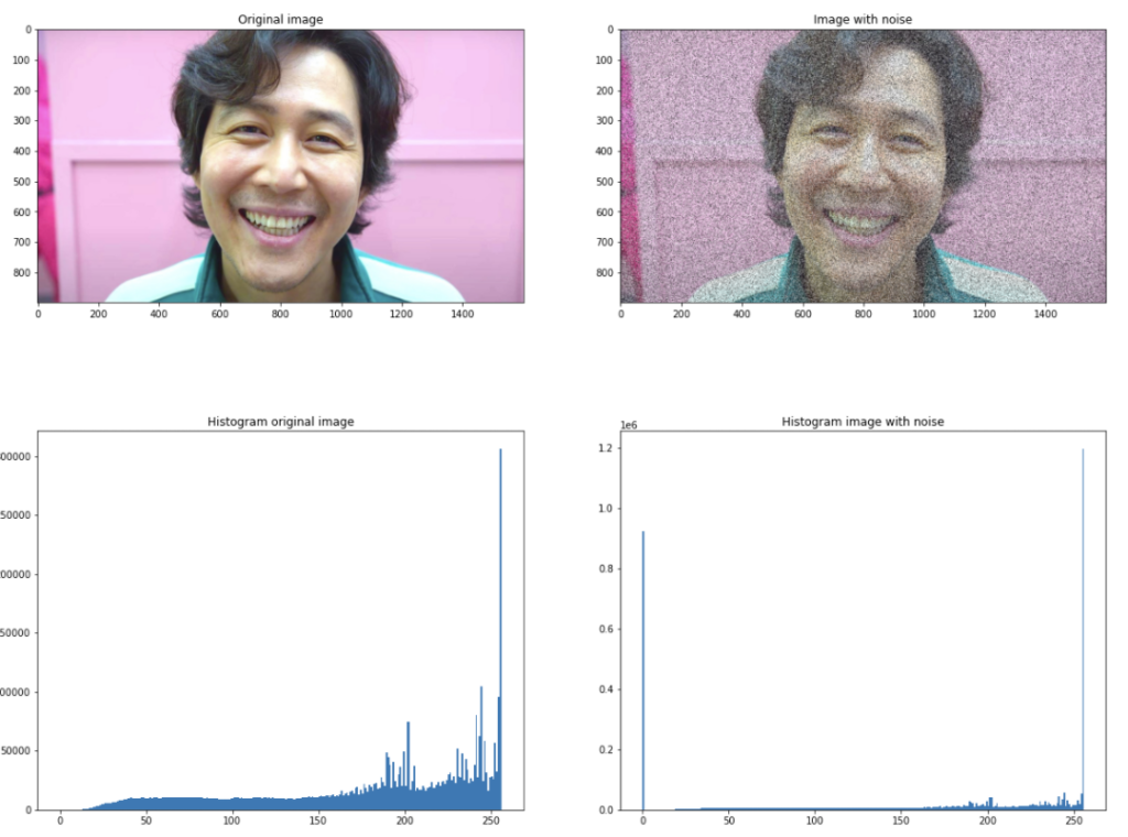
As we can see in the histogram on the right side, we got a lot of white and black pixels (bars at both ends of the histogram), so that means it has worked.
Fixing it
Now we will use the output image as input for the median filter. For that, we can make use of this function:
def median_filter(data, filter_size):
    """
        This function is the median filter algorigthm itself

        Parameters:
            data -- array containing the three RGB layers of an image
            filter_size -- size of the window to apply over the image
    """
    temp = []
    indexer = filter_size // 2
    data_filtered = np.zeros((len(data),len(data[0])))
    for i in range(len(data)):
        for j in range(len(data[0])):
            for z in range(filter_size):
                if i + z - indexer < 0 or i + z - indexer > len(data) - 1:
                    for c in range(filter_size):
                        temp.append(0)
                else:
                    if j + z - indexer < 0 or j + indexer > len(data[0]) - 1:
                        temp.append(0)
                    else:
                        for k in range(filter_size):
                            temp.append(data[i + z - indexer][j + k - indexer])

            temp.sort()
            data_filtered[i][j] = temp[len(temp) // 2]
            temp = []
    return data_filtered
But remember! as I mentioned before, the median filter works over a 2D image, in other words, a black and white image. Since we are using a full coloured image, we need to ‘separate’ the RGB channels and apply the median filter on each separately, said that, we will have now three different inputs:

In summary, this what we have done so far:

Now, it is time to filter each of the images resulting for the RGB channels, so the “cleaning” part of the pipeline will be:

Let’s do some zoom over the obtained image and check the results:

And there we go! this is the result of the image filtered. As you can see, there are still some contaminated pixels that could not be fixed by the filter. The reason why this happen is due to we may have chosen a window size very small (w=3), but we need to keep in mind that one of the disadvantages of bigger window sizes are that they will increase the ‘blurred’ effect over the filtered image.
That is one of the limitations of the standard median filter. There are some variations that produce much better results, like the called ‘adaptive median filter’ which is pretty much the same but with the difference that the window size can be different on each variation.
If you want to see it in action, leave a comment on this post! And as I always do, you have the full code available of this post on my Github repo, so check it out and feel free to use it for your proyects!
Cheers!